Editor’s note: Thanks to the diligence of Armin Grueneich this post has been amended to reflect the addition of step #5, below, in the calculation of the rescaled range.

Rescaled range analysis is a statistical technique designed to assess the nature and magnitude of variability in data over time. In investing rescaled range analysis has been used to detect and evaluate the amount of persistence, randomness, or mean reversion in financial markets time series data. Insight of this kind into financial data naturally suggests investment strategies.

Originally invented for the field of hydrology by Harold Edwin Hurst, the technique was developed to predict Nile River flooding in advance of the construction of the Aswan High Dam. The dam needed to fulfill multiple and divergent purposes, including serving as both a store of water to protect against drought for farmers down river, and as flood protection for those same farmers during typical annual flooding. Rainfall levels in Central Africa were seemingly random each year, yet the Nile River flows seemed to show autocorrelation. That is, rainfall in one time period seemed to influence rainfall in subsequent periods. Hurst needed to be able to see if there was a hidden long-term trend — statistically known as a long-memory process — in the Nile River data that might guide him in building a better dam for Egypt.

Does this sound familiar? A time series of varying levels that is seemingly random but in which it is suspected that there might also be a long-term, hidden trend. Not surprisingly rescaled range analysis had its moment in the financial analysis sun in the mid-1990s, when chaos theory, as applied to financial markets was a hot topic. Chaos theory is a branch of science that studies the interconnectedness of events that otherwise, on the surface, seem random.

Closely associated with rescaled range analysis is the Hurst exponent, indicated by H, also known as the “index of dependence” or the “index of long-range dependence.” A Hurst exponent ranges between 0 and 1, and measures three types of trends in a time series: persistence, randomness, or mean reversion.

• If a time series is persistent with H ≥ 0.5, then a future data point is likely to be like a data point preceding it. So an equity with H of 0.77 that has been up for the past week is more likely to be up next week as well, because its Hurst exponent is greater than 0.5.
• If the Hurst exponent of a time series is H < 0.5, then it is likely to reverse trend over the time frame considered. Thus, an equity with H = 0.26 that was up last month is more likely than chance to be down next month.
• Time series that have Hurst exponents near to 0.5 display a random (i.e., a stochastic) process, in which knowing one data point does not provide insight into predicting future data points in the series.

So what are the steps to conducting a rescaled range analysis and to estimating the Hurst exponent? As an instructional example, please reference the spreadsheet of the rescaled range analysis of daily return data for the S&P 500 Index from 3 January 1950 through 15 November 2012.

Rescaled Range Analysis Steps

1. Choose your time series. Do you want to analyze fluctuations in the yield curve? West Texas sweet crude? Apple (AAPL) or Google (GOOG) stock? Or the Dow Jones Industrial Average (DJIA)? Here I am going to select the S&P 500’s daily returns.

2. Choose your ranges. Rescaled range analysis depends on multiple lengths of time (i.e., ranges) to be analyzed and chosen arbitrarily by the analyst. In the example of the S&P 500, there are 15,821 daily returns. So I chose the following ranges, all powers of two:

a. Size of range is the entire data series = one range of 15,821 daily returns.

b. Size of each range is 1/2 of the entire data series = 15,821 ÷ 2 = two ranges of either 7,911 or 7,910 daily returns.

c. Size of each range is 1/4 of the entire data series = 15,821 ÷ 4 = four ranges of either 3,956 or 3,955 daily returns.

d. Size of each range is 1/8 of the entire data series = 15,821 ÷ 8 = eight ranges of either 1,978 or 1,977.

e. Size of each range is 1/16 of the entire data series = 15,821 ÷ 16 = sixteen ranges of either 989 or 988 daily returns.

f. Size of each range is 1/32 of the entire data series = 15,821 ÷ 32 = thirty-two ranges of either 495 or 494 daily returns.

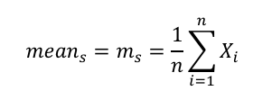
3. Calculate the mean for each range. For each of the ranges, calculate a mean per the formula below. Note: In the above example of the S&P 500 there are 1 + 2 + 4 + 8 + 16 + 32 = 63 means calculated, one for each range.

Where:

s = series (Series 1 is whole data series for S&P 500, or 15,821 daily returns; series 5 is 16 ranges of either 989 or 988 daily returns.)

n = the size of the range for which you are calculating the mean

X = the value of one element in the range

4. Create a series of deviations for each range. Create another time series of deviations using the mean for each range. Note: In the case of the S&P 500, there will be six new “deviations from the mean” ranges, given the six categories of ranges chosen in Step 2 above (i.e. ranges a, b, c, d, e, and f).

Where:

Y = the new time series adjusted for deviations from the mean

X = the value of one element in the range

m = the mean for the range calculated in Step 3 above

5. Create a series which is the running total of the deviations from the mean.  Now that you have a series of deviations from the mean for each range, you need to calculate a running total for each range’s deviations from the mean.

Where:

y = the running total of the deviations from the mean for each series

Y = the time series adjusted for deviations from the mean

6. Calculate the widest difference in the series of the running total of deviations from the mean. Find both the maximum and minimum values in the series of deviations for each range. Take the difference between the maximum and minimum in order to calculate the widest difference. Note: For the S&P 500 example, there are 63 calculations, one for each of the 63 ranges.

Where:

R = the widest spread in each range

Y = the value of one element in the “running total of deviations from the mean” range

7. Calculate the standard deviation for each range. Note: There will be 63 standard deviations, one for each range.

8. Calculate the rescaled range for each range in the time series. This step creates a new measure for each range in the time series that shows how wide is the range measured in standard deviations.

Where:

R/S = the rescaled range for each range in the time series

R = the range created in step 5 above

σ = the standard deviation for the range under consideration

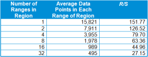
9. Average the rescaled range values for each region to summarize each range. For each region, average the rescaled range (R/S) values. Using the S&P 500 data as an example, we have the following R/S values for each of the four ranges of ~3,955 in size:

“Range 1/4”, part 1, R/S: 83.04

“Range 1/4”, part 2, R/S: 63.51

“Range 1/4”, part 3, R/S: 84.16

“Range 1/4”, part 4, R/S: 88.09

Average of the four R/S values for “Range 1/4” = (83.04 + 63.51 + 84.16 + 88.09) ÷ 4 = 79.70

For the S&P 500 we have the following values for the rescaled ranges:

Now that you have rescaled each range in the time series, you can calculate the Hurst exponent, H, that will summarize in one number the degree of persistence, randomness, or mean reversion in your time series.

Calculating the Hurst Exponent Steps

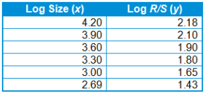
1. Calculate the logarithmic values for the size of each region and for each region’s rescaled range. For example, consider the above S&P 500 data:

2. Plot the logarithm of the size (x axis) of each series versus the logarithm of the rescaled range (y axis). This results in a graph that looks something like this one for the S&P 500:

Rescaled Range Analysis of the S&P 500 (3 January 1950 to 15 November 2012)

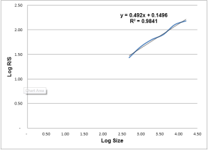
3. Calculate the slope of the data to find the Hurst exponent. H is the slope of the plot of each range’s log (R/S) versus each range’s log (size). For the S&P 500 for 3 January 1950 to 15 November, H is 0.49. Recall that this means that the S&P 500 demonstrates randomness.

Knowing the H, suggests some hypothetical trading strategies. For example, stocks with H ≥ 0.5 — that is, persistence — and positive price appreciation would be attractive to a growth manager wanting future capital appreciation. Whereas, stocks with H < 0.5 with prices declining for some time suggest an eventual price trend reversal to a value investor.

Photo credit: ©iStockphoto.com/ugurhan

Originally published on CFA Institute’s  Enterprising Investor.