Is the S&P 500 Mean Reverting? Rescaled Range Analysis Provides the Answer

Editor’s note: Thanks to the diligence of Armin Grueneich this post has been amended to reflect an additional step in the calculation of the rescaled range which has affected the prior reported results.

In a previous post, I used the S&P 500 as an example to demonstrate the use of a sophisticated quantitative method, rescaled range analysis, for evaluating whether a time series is random, persistent, or mean reverting. Rescaled range analysis was developed to spot trends hidden in the seeming randomness of African rainfall and its effect on Nile river flooding — but its application to investing yields many interesting insights.

Without much further explanation in my prior post, I stated that the S&P 500 had a Hurst exponent, H, of 0.49, for the time period 3 January 1950 to 15 November 2012. What does that mean? Is there greater granularity in the rescaled range analysis that reveals even more interesting findings? What other associated measures can be used to provide even greater insight?

First, let’s recap the basics. Recall that H takes on values between 0 and 1, and that a reading near 0.5 is representative of a randomly generated time series. Put another way, a data point in this kind of time series does not influence the result of another. Persistent time series are those with a Hurst exponent between 0.51 and 1.0, meaning that subsequent data is likely to take on the sign of preceding data. Data between 0.0 and 0.49 are mean reverting. In other words, subsequent data are likely to have an opposite directional sign from preceding data.

The S&P 500’s Hurst exponent of 0.49 is right near the ‘randomness’ center of 0.5 and only slightly on the mean reversion side of things. If we divide the Hurst exponent range into thirds — 0.00 to 0.33 for mean reverting, 0.34 to 0.67 for random, and 0.68 to 1.00 for persistence — a strong statement can be made that the S&P 500 is a random time series.

Index investing would have been a valuable strategy over the many years considered in the time series. Why? Because the time series is not predictable, though, on average the index generates a mean return of 0.03% daily (covered in yet another previous post).  So rescaled range analysis seems to have resolved the age old question of active versus passive investing!

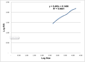
Well, not exactly. There is more information to behold in the data. Look at the chart below to see why we cannot quite crown value investing as the winning strategy.

Rescaled Range Analysis of the S&P 500 (3 January 1950 to 15 November 2012)

While there is a very high r-squared for the regression line — 0.98 — the actual data ‘wiggle.’ You see rescaled range analysis and the Hurst exponent are ways of looking at the self-similarity, or autocorrelation, of data. When rescaled range analysis is conducted, data are divided into ever smaller ranges. Those smaller ranges are then evaluated to see if the relationships detected for the whole data series are present in smaller time scales, too. Incidentally, this is why this type of analysis is favored by chaos theoreticians, who also focus on self-similarity and scalability of phenomenon in hard science data.

As you can see from the graph, randomness does not hold for all of the time scales. So what do they say? They say that for the first half of its history the S&P 500 showed persistence with daily returns for the S&P 500 having a Hurst exponent of 0.61 — in the realm between random and persistent.  Whereas, in the second half of its existence the S&P 500 is actually more random with a Hurst exponent of 0.46.  This suggests two very different types of investment environments over the long history of the S&P 500.  It would be interesting to corroborate the experience of traders from many decades ago with the preceding result and to compare them with veterans of a more recent era.

How long are these time scales since we are looking at lognormal data? The time frames are precisely 7,911 trading days (31.39 years!) up to the full 15,821 trading days examined. Put another way, over the very long run growth investors would have benefited as subsequent periods are of the same sign as preceding periods: up.

Finally, in Euclidean geometry a straight line — i.e., a time series with no variation in our case — is considered to have a topological dimension of 1, whereas a square is a 2-dimensional surface and a cube is a three-dimensional object. Yet financial market data do not unfold in a straight line, and in fact the rougher they are the more closely they approach being a surface of two dimensions. A measure for the smoothness/roughness of data is the fractal dimension and is calculated as D = 2 – Hurst Exponent.

For the S&P 500, the fractal dimension for the entire time series is 2 – 0.49 = 1.51. In other words, the time series line of daily returns for the S&P 500 is fairly rough. Yet, at shorter time frames, as discussed above, the fractal dimension fluctuates between 1.39, calculated as 2 – 0.61, and 1.54, calculated as 2 – 0.46.

All of this is a quantitative way to communicate a qualitative message: The S&P 500 is a volatile time series. Caveat emptor!

Photo credit: ©iStockphoto.com/luchschen

Originally published on CFA Institute’s  Enterprising Investor.